41 conditional formatting data labels excel
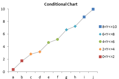
Conditional formatting chart data labels? - Excel Help Forum You have to format all axis tick labels the same. You can use a dummy line chart series to add data labels which can be individually formatted, as I explain in Individually Formatted Category Axis Labels. The easy way to conditionally format these labels is use two series. Use something like =IF ($E2=1,0,NA ()) for the series that has red labels How-to Make Conditional Data Labels for an Excel Dashboard Checkout the Step-by-Step Tutorial here: on How to conditionally hide and unhide data labels ...
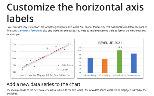
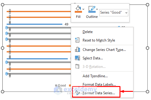
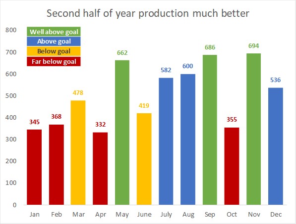
Excel bar chart with conditional formatting based on MoM change Initial formatting The initial formatting cleans up the chart and gets it ready for the labels. Start by reversing the order of the bars. Select the vertical axis and press Ctrl+1 to make the Format Axis task pane appear. In the Axis Options section, check the "Categories in reverse order" checkbox.

Conditional formatting data labels excel
Excel Data Analysis - Conditional Formatting - tutorialspoint.com Follow the steps to conditionally format cells − Select the range to be conditionally formatted. Click Conditional Formatting in the Styles group under Home tab. Click Highlight Cells Rules from the drop-down menu. Click Greater Than and specify >750. Choose green color. Click Less Than and specify < 500. Choose red color. Use conditional formatting to highlight information - Microsoft Support The default method of scoping fields in the Values area is by selection. You can change the scoping method to the corresponding field or value field by using the Apply formatting rule tooption button, the New Formatting Ruledialog box, or the Edit Formatting Ruledialog box. Use Quick Analysis to apply conditional formatting Conditional Formatting in Excel (Complete Guide + Examples) What is Conditional Formatting. Conditional Formatting is a feature in Excel that changes the display of cells whose values meet the Conditional Formatting rule's criterion.Conditional Formatting makes it very easy to make note of important data whether numerical or non-numerical.. This feature uses graphic means such as highlighting, icons, and data bars to visually cast attention on the ...
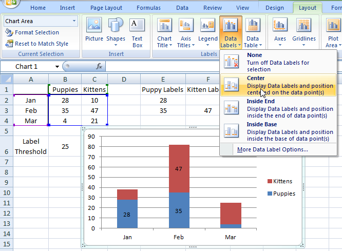
Conditional formatting data labels excel. › conditionalConditional formatting for Excel column charts | Think ... Additional formatting. The colors used for each data series is from the color theme being used for this Excel file. You can assign more meaningful colors for each data series. You can also add data labels to each series. It is a good idea to format the data label text to have the same color as the column it is representing. How to Create Excel Charts (Column or Bar) with Conditional Formatting ... Right-click on any of the columns and pick " Format Data Series " from the contextual menu that pops up. In the task pane, change the position and width of the columns: Switch to the Series Options tab. Change " Series Overlap " to " 100%. " Set the Gap Width to " 60%. " Step #4: Adjust the color scheme. At last, add the final touches. Creating Conditional Data Labels in Excel Charts - YouTube We can make labels appear on our charts that don't have to do with the raw numbers that built the chart - and we can make them show up or not based on whatever conditions we want. In this... Hasaan Fazal on LinkedIn: Conditional Format Data labels in Excel ... Conditional Format Data labels in Excel: Colors and Symbols - Change Data Label…
Conditional Formatting with Data Validation - Microsoft Community Hub I am trying to have a cell be red if other criteria is met on other cells. For example, if A2=Value, B2= Value, and C2 is blank, I would like to have C2 turn red. A2,B2, and C2 all have a list range for the Data Validation. For the conditional formatting, I have only put the range to apply to as column C. How to Use Conditional Formatting to Highlight Text in Excel - Spreadsheeto 2. In the middle of the Home tab, click 'Conditional Formatting'. 3. Hover your cursor over 'Highlight Cells Rules' and select 'Text that Contains'. 4. In the dialog box that appears, write the text you want to highlight, in the left field. As you type it, you can see the conditional formatting applied instantly. Conditional Formatting to Distinguish Between Labels and Numbers I want to conditionally format each cell, so that the text is yellow, the numbers are blue, and the blank cells are green. I tried by setting up a new rule under conditional formatting, then selecting "use a formula to determine which cells to format", then using some combinations of the if, istext, isnumber, etc. combinations. Please advise. Conditional Formatting in Excel - Step by Step Examples - WallStreetMojo Step 1: Select the range A5:A19 on which conditional formatting is to be applied. Subsequently, from the "conditional formatting" drop-down (in the Home tab), choose "highlight cells rules." Next, select "greater than." Step 2: The "greater than" window opens, as shown in the following image. Under "format cells that are greater than," enter 30.
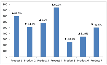
VBA Conditional Formatting of Charts by Value and Label The first series of the active chart is defined as the series we are formatting. The category labels (XValues) and values (Values) are put into arrays, also for ease of processing. The code then looks at each point's value and label, to determine which cell has the desired formatting. The rows and columns are looped starting at 2, since the ... Conditional Formatting in Excel (Easy Tutorial) Formulas that apply conditional formatting must evaluate to TRUE or FALSE. 1. Select the range A1:E5. 2. On the Home tab, in the Styles group, click Conditional Formatting. 3. Click New Rule. 4. Select 'Use a formula to determine which cells to format'. 5. Enter the formula =ISODD (A1) 6. Select a formatting style and click OK. Result. Custom Data Labels with Colors and Symbols in Excel Charts - [How To ... Step 4: Select the data in column C and hit Ctrl+1 to invoke format cell dialogue box. From left click custom and have your cursor in the type field and follow these steps: Press and Hold ALT key on the keyboard and on the Numpad hit 3 and 0 keys. Let go the ALT key and you will see that upward arrow is inserted. Excel Conditional Formatting How-To | Smartsheet From the Home tab, click Conditional Formatting on the right side of the toolbar, and click Highlight Cells Rules from the dropdown menu. Click Less than . A box will appear. Type 100 in the empty field. Click OK . Your spreadsheet will now reflect this highlight rule, with the quantities less than 100 highlighted red with red text.
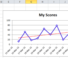
Highlight Max & Min Values in an Excel Line Chart - Xelplus ...
How to do conditional formatting of a label in Excel VBA Function ConditionalFormatNumber (n As Double) As String If n > 1000000 Then ConditionalFormatNumber = Format (n / 1000000, "$#,##0.00,,""M""") ElseIf n > 1000 Then ConditionalFormatNumber = Format (n / 1000, "$#,##0.00, ""K""") Else ConditionalFormatNumber = Format (n, "$#,##0.0") End If End Function Share Improve this answer Follow
Format Chart Numbers as Thousands or Millions — Excel ...
peltiertech.com › prevent-overlapping-data-labelsPrevent Overlapping Data Labels in Excel Charts - Peltier Tech May 24, 2021 · Overlapping Data Labels. Data labels are terribly tedious to apply to slope charts, since these labels have to be positioned to the left of the first point and to the right of the last point of each series. This means the labels have to be tediously selected one by one, even to apply “standard” alignments.

How to create a chart with conditional formatting in Excel?
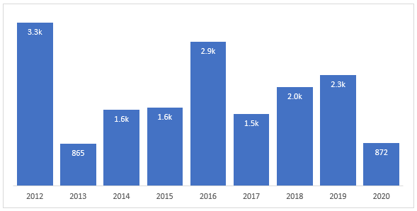
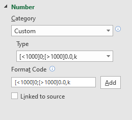
techcommunity.microsoft.com › t5 › excel-blogMicrosoft Excel conditional number formatting Sep 17, 2019 · Next, I would apply conditional formatting number formatting where the cell value is greater than one so that numbers greater than a million could be displayed to the nearest 0.1m, numbers less than a million but greater than or equal to 1,000 could be displayed to the nearest 0.00k and numbers lower than 1,000 (but necessarily greater than one ...
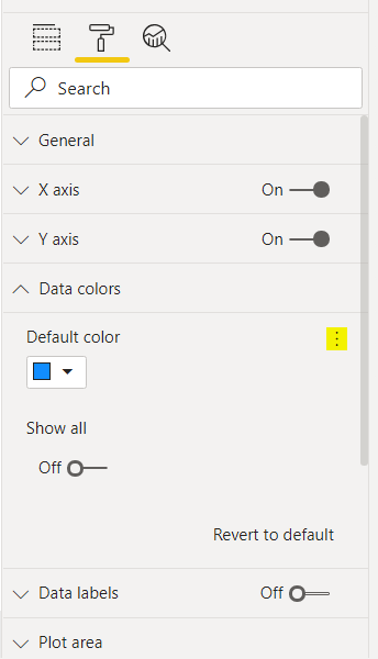
Power BI: Conditional formatting and data colors in action
› conditional-formatting-in-pivot-tableExcel Conditional Formatting in Pivot Table - EDUCBA For applying conditional formatting in this pivot table, follow the below steps: Select the cells range for which you want to apply conditional formatting in excel. We have selected the range B5:C14 here. Go to the HOME tab > Click on Conditional Formatting option under Styles > Click on Highlight Cells Rules option > Click on Less Than option.

Conditional formatting for Data Labels in Power BI - Power BI ...
How to create a chart with conditional formatting in Excel? - ExtendOffice Select the chart you want to add conditional formatting for, and click Kutools > Charts > Color Chart by Value to enable this feature. 2. In the Fill chart color based on dialog, please do as follows: (1) Select a range criteria from the Data drop-down list; (2) Specify the range values in the Min Value or Max Value boxes; (3) Choose a fill ...

Upgrading Your Data Labels With Conditional Formatting!
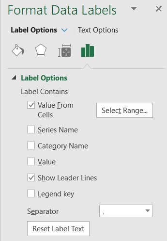
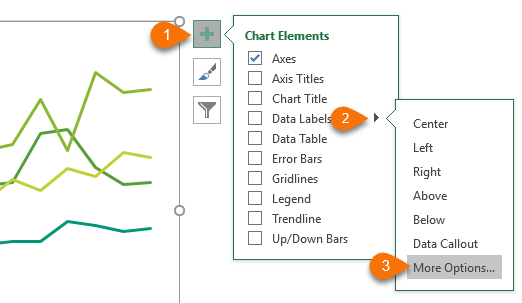
Change the format of data labels in a chart - Microsoft Support To get there, after adding your data labels, select the data label to format, and then click Chart Elements > Data Labels > More Options. To go to the appropriate area, click one of the four icons ( Fill & Line, Effects, Size & Properties ( Layout & Properties in Outlook or Word), or Label Options) shown here.

Conditional Formatting (Fill Color, Font Color etc...) for ...
How to change chart axis labels' font color and size in Excel? You can get it done with conditional formatting easily as follows: 1. Right click the axis you will change labels by positive/negative/0, and select the Format Axis from right-clicking menu. 2. Do one of below processes based on your Microsoft Excel version:

Conditional formatting for Data Labels in Power BI - Power BI ...
A Quick Guide to Conditional Formatting in Excel - HubSpot 1. Start by selecting the cell (or cell range) that contains a conditional formatting rule. 2. Navigate to the header toolbar and select Conditional Formatting, then Manage Rules. 3. The Manage Rules dialog box will list the current rules for your selection. Select the rule you want to edit and click Edit Rule.

Custom Data Labels with Colors and Symbols in Excel Charts ...
How to Use Conditional Formatting Based on Date in Microsoft Excel Open the sheet, select the cells you want to format, and head to the Home tab. In the Styles section of the ribbon, click the drop-down arrow for Conditional Formatting. Move your cursor to Highlight Cell Rules and choose "A Date Occurring" in the pop-out menu. A small window appears for you to set up your rule.
Format Chart Numbers as Thousands or Millions — Excel ...
techcommunity.microsoft.com › t5 › excelConditional formatting for entire row based on data in one ... Jul 30, 2019 · I need all cells in a row to highlight a certain color if the data in one cell contains a specific word. What I specifically want is for an entire row to turn grey if the status cell contains the word "SHIPPED." I know how to make that specific cell highlight the color I want, but not the entire ...

How to: Display and Format Data Labels | .NET File Format ...
Conditional formatting for Data Labels in Power BI Step-1: Select the visual >go to the format pane>Data Labels. Step-2: Choose measure from "Apply settings to". choose measure Step-3: Go to Values> Click on fx icon. Step-4: Choose Format Style - Rules and Select measure name. After that add rules condition, see the below given screen shot. Choose Rules conditional formatting

Excel Custom Chart Labels • My Online Training Hub
Conditional Formatting in Excel - The Complete Guide | Layer Blog Select your cell range and go to Conditional Formatting > New Rule. Conditional Formatting in Excel - Create New Rule. 2. A dialog box will pop up. Select "Classic" in the "Style" field, and "Use a formula…" from the drop-down menu. Conditional Formatting in Excel - New formatting rule options. 3.

How to Get Colors in Excel Chart Data Lables - Formatting Trick
› Conditional-formatting-ExcelConditional Formatting in Excel - a Beginner's Guide Excel has a tool that automatically helps you out with that — it’s called conditional formatting. If you’re ready to take your data organization game to the next level, keep reading to learn how to use conditional formatting in Excel. In this resource, we'll apply conditional formatting to a pivot table. Note that the steps to apply pivot ...
Conditionally format data labels - Excel Charts
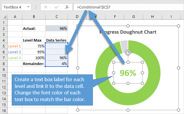
› charts › progProgress Doughnut Chart with Conditional Formatting in Excel Mar 24, 2017 · Great question! The Excel Web App does not support those text box shapes yet. We can use the built-in data labels for the chart instead. The label for the Remainder bar can be deleted by left clicking on the label twice, then pressing the delete key. That just leaves the data label for the actual progress amount. Here is a screenshot.
Microsoft Excel 365 Chart tips and tricks
Apply conditional table formatting in Power BI - Power BI In the Visualizations pane, right-click or select the down-arrow next to the field in the Values well that you want to format. Select Conditional formatting, and then select the type of formatting to apply. Note Conditional formatting overrides any custom background or font color you apply to the conditionally formatted cell.

How to improve or conditionally format data labels in Power ...
Format Data Labels in Excel- Instructions - TeachUcomp, Inc. To format data labels in Excel, choose the set of data labels to format. To do this, click the "Format" tab within the "Chart Tools" contextual tab in the Ribbon. Then select the data labels to format from the "Chart Elements" drop-down in the "Current Selection" button group.

Conditional formatting for Data Labels in Power BI - Power BI ...
Conditional Formatting in Excel (Complete Guide + Examples) What is Conditional Formatting. Conditional Formatting is a feature in Excel that changes the display of cells whose values meet the Conditional Formatting rule's criterion.Conditional Formatting makes it very easy to make note of important data whether numerical or non-numerical.. This feature uses graphic means such as highlighting, icons, and data bars to visually cast attention on the ...
Apply Conditional Formatting to Chart Data Labels
Use conditional formatting to highlight information - Microsoft Support The default method of scoping fields in the Values area is by selection. You can change the scoping method to the corresponding field or value field by using the Apply formatting rule tooption button, the New Formatting Ruledialog box, or the Edit Formatting Ruledialog box. Use Quick Analysis to apply conditional formatting

Apply Custom Conditional Formatting to Clustered Column Chart ...
Excel Data Analysis - Conditional Formatting - tutorialspoint.com Follow the steps to conditionally format cells − Select the range to be conditionally formatted. Click Conditional Formatting in the Styles group under Home tab. Click Highlight Cells Rules from the drop-down menu. Click Greater Than and specify >750. Choose green color. Click Less Than and specify < 500. Choose red color.
Excel bar chart with conditional formatting based on MoM ...

Solved: Conditional Formatting of Bar Chart - Microsoft Power ...
Excel Bar Graph Color with Conditional Formatting (3 Suitable ...

Solved: Conditional Formatting Data Labels - Microsoft Power ...
How-to Make Conditional Label Values in an Excel Stacked ...
Conditional Formatting of Excel Charts - Peltier Tech

Solved: Conditional Formatting of Bar Chart - Microsoft Power ...

Custom Excel Chart Label Positions • My Online Training Hub
How to Create Excel Charts (Column or Bar) with Conditional ...

Creating Conditional Data Labels in Excel Charts | Everyday Office 075

Apply Custom Data Labels to Charted Points - Peltier Tech
Progress Doughnut Chart with Conditional Formatting in Excel ...
Conditional formatting for Excel column charts | Think ...
Dynamically Label Excel Chart Series Lines • My Online ...

Apply Custom Data Labels to Charted Points - Peltier Tech

Conditional Formatting of Data Labels on Chart - Microsoft ...
Show Trend Arrows in Excel Chart Data Labels
How to change chart axis labels' font color and size in Excel?

Dynamic Number Format for Millions and Thousands - PK: An ...

Custom data labels in a chart

Custom data labels in a chart

Conditional Formatting of Data Labels on Chart - Microsoft ...
Post a Comment for "41 conditional formatting data labels excel"