40 excel bar graph labels
2 data labels per bar? - Microsoft Community Replied on January 25, 2011 Use a formula to aggregate the information in a worksheet cell and then link the data label to the worksheet cell. See Data Labels Tushar Mehta (Technology and Operations Consulting) (Excel and PowerPoint add-ins and tutorials) How to Add Percentages to Excel Bar Chart If we would like to add percentages to our bar chart, we would need to have percentages in the table in the first place. We will create a column right to the column points in which we would divide the points of each player with the total points of all players. We will select range A1:C8 and go to Insert >> Charts >> 2-D Column >> Stacked Column:
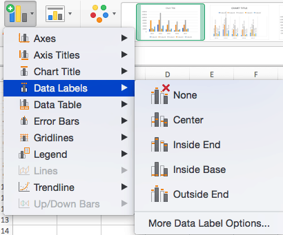
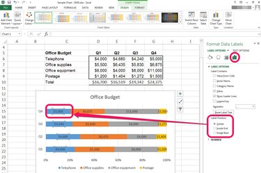
How to Create a Bar Chart With Labels Inside Bars in Excel 7. In the chart, right-click the Series "# Footballers" Data Labels and then, on the short-cut menu, click Format Data Labels. 8. In the Format Data Labels pane, under Label Options selected, set the Label Position to Inside End. 9. Next, in the chart, select the Series 2 Data Labels and then set the Label Position to Inside Base.
Excel bar graph labels
How to Create Bar Chart in Excel? - EDUCBA Step 1: Select the data > Go to Insert > Bar Chart > Cone Chart. Step 2: Click on the CONE chart, and it will insert the basic chart for you. Step 3: Now, we need to modify the chart by changing its default settings. Remove gridlines of the above Chart. Change the chart title to Sales by month. How to Make a Bar Chart in Microsoft Excel To add axis labels to your bar chart, select your chart and click the green "Chart Elements" icon (the "+" icon). From the "Chart Elements" menu, enable the "Axis Titles" checkbox. Axis labels should appear for both the x axis (at the bottom) and the y axis (on the left). These will appear as text boxes. How to Change Excel Chart Data Labels to Custom Values? Go to Formula bar, press = and point to the cell where the data label for that chart data point is defined. Repeat the process for all other data labels, one after another. See the screencast. Points to note: This approach works for one data label at a time. So if you have a large chart, you are in for a lot of clicks and manic mouse maneuvering.
Excel bar graph labels. Bar Chart Target Markers - Excel University The first step is to insert the chart. Insert clustered bar chart. Select any cell in the data table and select Insert > Clustered Bar chart. We then remove the legend and gridlines, and update the title. At this point, our chart displays sales with blue bars, forecast values with orange bars, and looks a bit like this: How to place labels underneath bar chart - Microsoft Community Answer jpgpinto Replied on February 20, 2012 The names are appearing below the chart axis, that is on value 0.0%. They are on the correct place. If you want them to appear at the bottom of your chart, just select the axis and on the "Format axis" dialog box, on the "Axis options" tab, on the "Axis labels:" option, select "Low". jpgpinto Histogram with Actual Bin Labels Between Bars - Peltier Tech Select the chart, then use Home tab > Paste dropdown > Paste Special to add the copied data as a new series, with category labels in the first column. You don't see the new series, because it's a series of bars with zero height. But you should notice that the wide bars have been squeezed a bit to make room for the added series. How to Use Cell Values for Excel Chart Labels Select the chart, choose the "Chart Elements" option, click the "Data Labels" arrow, and then "More Options." Uncheck the "Value" box and check the "Value From Cells" box. Select cells C2:C6 to use for the data label range and then click the "OK" button. The values from these cells are now used for the chart data labels.
How to Insert Axis Labels In An Excel Chart | Excelchat We will go to Chart Design and select Add Chart Element Figure 6 - Insert axis labels in Excel In the drop-down menu, we will click on Axis Titles, and subsequently, select Primary vertical Figure 7 - Edit vertical axis labels in Excel Now, we can enter the name we want for the primary vertical axis label. How to Add Axis Labels in Excel Charts - Step-by-Step (2022) If you would only like to add a title/label for one axis (horizontal or vertical), click the right arrow beside 'Axis Titles' and select which axis you would like to add a title/label. Editing the Axis Titles After adding the label, you would have to rename them yourself. There are two ways you can go about this: Manually retype the titles Edit titles or data labels in a chart - support.microsoft.com The first click selects the data labels for the whole data series, and the second click selects the individual data label. Right-click the data label, and then click Format Data Label or Format Data Labels. Click Label Options if it's not selected, and then select the Reset Label Text check box. Top of Page Text Labels on a Horizontal Bar Chart in Excel - Peltier Tech On the Excel 2007 Chart Tools > Layout tab, click Axes, then Secondary Horizontal Axis, then Show Left to Right Axis. Now the chart has four axes. We want the Rating labels at the bottom of the chart, and we'll place the numerical axis at the top before we hide it. In turn, select the left and right vertical axes.
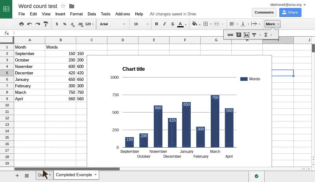
How to Create a Bar Chart With Labels Above Bars in Excel In the chart, right-click the Series "Dummy" Data Labels and then, on the short-cut menu, click Format Data Labels. 15. In the Format Data Labels pane, under Label Options selected, set the Label Position to Inside End. 16. Next, while the labels are still selected, click on Text Options, and then click on the Textbox icon. 17. Excel: How to Create a Bubble Chart with Labels - Statology Step 3: Add Labels. To add labels to the bubble chart, click anywhere on the chart and then click the green plus "+" sign in the top right corner. Then click the arrow next to Data Labels and then click More Options in the dropdown menu: In the panel that appears on the right side of the screen, check the box next to Value From Cells within ... Bar Chart in Excel | Examples to Create 3 Types of Bar Charts We will add "Data Labels" to the data series in the plotted area. We will click on the chart area to select the data series. Now, as shown in the screenshot, we will right-click on the data series and choose the add data labels to add the data label option. We can move the bar chart to the desired place in the worksheet. Create a multi-level category chart in Excel - ExtendOffice Select the dots, click the Chart Elements button, and then check the Data Labels box. 23. Right click the data labels and select Format Data Labels from the right-clicking menu. 24. In the Format Data Labels pane, please do as follows. 24.1) Check the Value From Cells box;
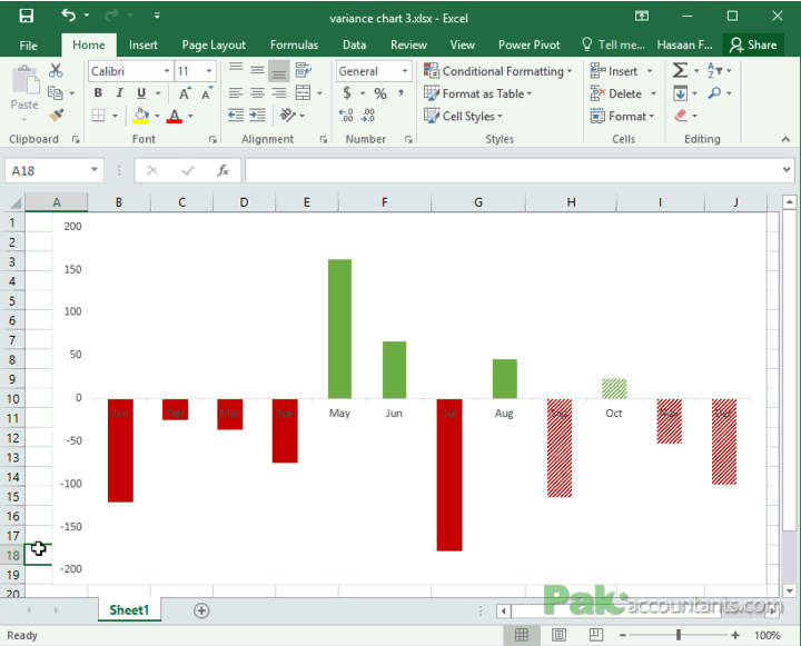
Moving X-axis labels at the bottom of the chart below negative values in Excel - PakAccountants.com
Clustered Bar Chart in Excel - WallStreetMojo Then, click on the "Column Chart" button in the "Charts" group and select a chart from the drop-down menu. Select the third column chart (called clustered bar) in the "2-D Bar" column section. Once we select a chart type, Excel will automatically create the chart and insert it into our worksheet.
How to Make Charts and Graphs in Excel | Smartsheet
Bar Graph in Excel — All 4 Types Explained Easily To create a simple bar graph, follow these steps: Get your Data ready. Make sure it has one categorical variable and one quantitative secondary variable. In my example from Sheet1, I have the time duration of 6 tasks. Select your Data with headers. Locate and click on the 2-D Clustered Bars option under the Charts group in the Insert Tab.

Line Graph, Bar Graph, Scatter, Etc. | University of Denver
How to Make a Bar Graph in Excel: 9 Steps (with Pictures) 2. Click the Insert tab. It's in the editing ribbon, just right of the Home tab. 3. Click the "Bar chart" icon. This icon is in the "Charts" group below and to the right of the Insert tab; it resembles a series of three vertical bars. 4. Click a bar graph option.

Do My Excel Blog: How to design a multiple clustered bar chart series in Excel
How do I make excel label every bar in a bar chart? - Super User Here is what I have done: Insert->Pivot Chart Click Clustered Column Right-click on graph, select Format Axis set specify unit interval to 1 Excel now just labels every 2nd bar, even though it would easily fit (I have about 150 bars) with the given label font size.
/simplexct/images/Fig10-lfa95.jpg)
How to Create a Bar Chart With Labels Above Bars in Excel
How to label graphs in Excel | Think Outside The Slide I suggest placing them inside the end of the column or bar, or just outside the column or bar. This example shows a column graph with data labels only. Example 1. If the message is more related to the ranking of the values, then you can use an axis. You don't need data labels, the axis gives the audience the scale they need to compare the values.
Add labels to a Google chart or graph - YouTube
How to Add Total Data Labels to the Excel Stacked Bar Chart For stacked bar charts, Excel 2010 allows you to add data labels only to the individual components of the stacked bar chart. The basic chart function does not allow you to add a total data label that accounts for the sum of the individual components. Fortunately, creating these labels manually is a fairly simply process.

Advanced Graphs Using Excel : 3D-histogram in Excel
Excel charts: add title, customize chart axis, legend and data labels Click anywhere within your Excel chart, then click the Chart Elements button and check the Axis Titles box. If you want to display the title only for one axis, either horizontal or vertical, click the arrow next to Axis Titles and clear one of the boxes: Click the axis title box on the chart, and type the text.

How to Create Bar Graph in Microsoft Excel?
Add or remove data labels in a chart - support.microsoft.com Add data labels to a chart Click the data series or chart. To label one data point, after clicking the series, click that data point. In the upper right corner, next to the chart, click Add Chart Element > Data Labels. To change the location, click the arrow, and choose an option.

Excel - 2-D Bar Chart - Change horizontal axis labels - Super User
How to add data labels from different column in an Excel chart? Right click the data series in the chart, and select Add Data Labels > Add Data Labels from the context menu to add data labels. 2. Click any data label to select all data labels, and then click the specified data label to select it only in the chart. 3.

How to Create Bar Charts in Excel
How to Change Excel Chart Data Labels to Custom Values? Go to Formula bar, press = and point to the cell where the data label for that chart data point is defined. Repeat the process for all other data labels, one after another. See the screencast. Points to note: This approach works for one data label at a time. So if you have a large chart, you are in for a lot of clicks and manic mouse maneuvering.
/simplexct/images/Fig12-lc3b4.jpg)
How to Create a Bar Chart With Labels Above Bars in Excel
How to Make a Bar Chart in Microsoft Excel To add axis labels to your bar chart, select your chart and click the green "Chart Elements" icon (the "+" icon). From the "Chart Elements" menu, enable the "Axis Titles" checkbox. Axis labels should appear for both the x axis (at the bottom) and the y axis (on the left). These will appear as text boxes.
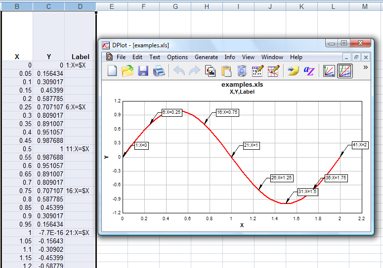
DPlot Windows software for Excel users to create presentation quality graphs
How to Create Bar Chart in Excel? - EDUCBA Step 1: Select the data > Go to Insert > Bar Chart > Cone Chart. Step 2: Click on the CONE chart, and it will insert the basic chart for you. Step 3: Now, we need to modify the chart by changing its default settings. Remove gridlines of the above Chart. Change the chart title to Sales by month.
How to Use Excel to Make a Percentage Bar Graph | Techwalla

35 How To Label Bar Graph In Excel - Best Labeling Ideas

How to add data labels to a Column (Vertical Bar) Graph in Microsoft® Excel 2013 - YouTube

How to Add Data Labels to your Excel Chart in Excel 2013 - YouTube

How to Make a Bar Graph in Excel: 10 Steps (with Pictures)

How to label graphs in Excel | Think Outside The Slide
Post a Comment for "40 excel bar graph labels"